Inventory optimization: setting safety stock and reorder points for every item with AI
Inventory optimization sets three numbers for each item: the safety stock, the reorder point and the order quantity. The goal is to reach the service level you choose with the least money tied up in stock. The settings come from data most businesses never measure item by item: how much demand varies, how much supplier lead times vary, and how often you can afford to run out. This guide gives the formulas, a calculator and what AI changes.

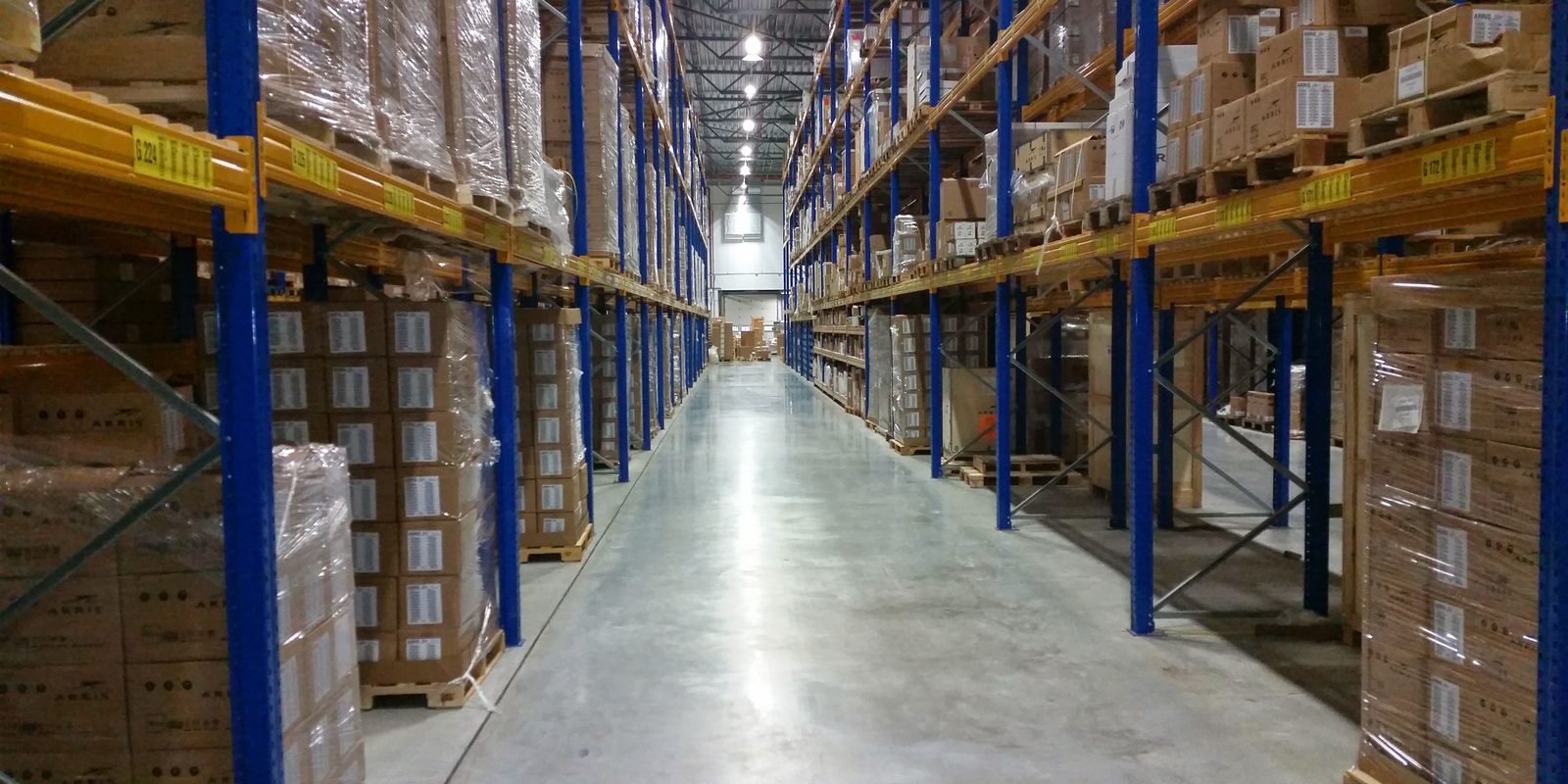
What inventory optimization is
Static rules give every item the same treatment, such as a month of cover. Inventory optimization sets each item from its own data and resets it when the data changes. The Business Development Bank of Canada (BDC) calls this a dynamic system in its guide to optimizing inventory management. In such a system, “reordering quantities and timing vary for each product based on its sales volume, lead time and safety stock level.”
The money involved is large. US businesses held $2,764.7 billion of inventory at the end of July 2026, according to the Census Bureau’s Manufacturing and Trade Inventories and Sales report, an inventories-to-sales ratio of 1.30.
Inventory forecasting, the demand forecast for each item, is the input to all of this. AI demand forecasting covers how to build it, and AI for inventory management covers the other inventory jobs, such as cycle counts and slow-moving stock. This guide covers what to do with the forecast.
How it is done by hand
Most smaller companies set stock levels with rules of thumb:
- The same weeks of cover for every item.
- Min/max levels set when the item was created and rarely changed.
- The lead time the supplier quotes, in place of the time orders actually take.
- Order quantities set by habit or by the supplier’s price break.
The result is too much of some items and too little of others. Two weeks of cover protects a steady seller well and an erratic one poorly. AI for inventory management shows how a reorder point built on a quoted lead time of 10 days runs out before the order lands when orders really take 14.
The inventory optimization formulas
The standard method comes from operations research. MIT’s Center for Transportation and Logistics sets out each piece in its supply chain key concepts, and the steps below follow it.
Service level
Choose the measure first. Cycle service level is “the probability that there will not be a stock out within a replenishment cycle.” Item fill rate is “the fraction of demand that is met with the inventory on hand out of cycle stock.” They differ, and MIT notes that fill rate “is always higher than CSL for the same safety stock level.” The cycle service level sets the safety factor k. With the normal distribution, k is about 1.645 for 95% and about 2.326 for 99%, values you can check in NIST’s table of the standard normal distribution.
Safety stock and reorder point
Safety stock is k times the standard deviation of demand over the lead time. The reorder point adds the expected demand over the lead time. When both demand and lead time vary, MIT combines the two sources of variation:
| Quantity | Formula |
|---|---|
| Demand over the lead time | Average daily demand × average lead time in days |
| Variation of demand over the lead time | σDL = √(average lead time × σD² + average daily demand² × σL²) |
| Safety stock | k × σDL |
| Reorder point | Demand over the lead time + safety stock |
Here σD is the standard deviation of daily demand and σL is the standard deviation of the lead time in days. Use the same time unit throughout.
Take an item that sells 8 units a day on average, with a standard deviation of 3 units a day and an average lead time of 14 days. The table compares a supplier that always takes 14 days with one whose lead time varies with a standard deviation of 3 days.
| Lead time never varies | Lead time varies by 3 days | |
|---|---|---|
| Demand over the lead time | 112 units | 112 units |
| Variation over the lead time (standard deviation) | 11.2 units | 26.5 units |
| Safety stock at 95% (k = 1.645) | 18.5 units | 43.6 units |
| Reorder point at 95% | 130.5 units | 155.6 units |
| Safety stock at 99% (k = 2.326) | 26.1 units | 61.6 units |
The supplier’s variation more than doubles the safety stock. Moving from 95% to 99% raises it by another 41%. MIT’s notes warn that “as k increases, it gets difficult to improve CSL and it will require enormous amount of inventory to cover the extreme limits.”
Order quantity
The order quantity sets how often you reorder. The economic order quantity (EOQ) balances the cost of placing an order against the cost of holding stock: EOQ = √(2 × cost per order × annual demand ÷ holding cost per unit per year). MIT calls it “exceptionally robust,” because ordering 50% more than the optimal quantity raises the relevant cost by only about 8%. It assumes steady demand, so treat it as a starting point and round it to the supplier’s pack sizes and minimums. AI in procurement covers turning the resulting suggestions into purchase orders.
If you order on a fixed day, such as every Monday, the stock must also cover the time until the next order. MIT notes that periodic review policies are popular “because they fit the regular pattern of work where ordering might occur only once a week or once every two weeks.” In the formulas above, replace the lead time with the lead time plus the review period.
Safety stock calculator
Enter your own numbers. The calculator runs in this browser tab, and nothing you type is sent anywhere or recorded. It uses the formulas above with the cycle service level you choose.
The calculator assumes demand is roughly normal, which suits items that sell on most days. For items that sell a few units a month, it overstates the precision, and the section on risks covers what to use instead.
What AI changes
The formulas stay the same. AI changes the quality and the freshness of the numbers that go into them, item by item.
It measures variation for every item
The formulas need the variation of demand and of lead time for each item, which is exactly what nobody measures by hand. Software computes both from order and receipt history, by item and by supplier, and refreshes them every month. MIT adds that σDL “is more technically the root mean square error (RMSE) of the forecast over the lead time.” A better forecast therefore lowers the safety stock you need.
It handles the items the formula fits badly
The normal formula fits items that sell on most days. For slow and lumpy items, software can replay your own history, order by order, to see how much demand arrives during a typical lead time. It can also use a probabilistic forecast that predicts the range directly. Google’s TimesFM-3, for example, predicts nine quantiles. The reorder point then becomes a percentile of demand over the lead time, such as the 95th.
It sets the service level by class
Not every item deserves 99%. A common approach groups items by value and by how steady their demand is, then sets a service level for each group. MIT measures steadiness with the coefficient of variation, “the standard deviation over the mean.” BDC describes its top class as “items you can’t afford to be out of stock ever.” Software keeps each item in the right group as its sales change. For items at the bottom of every ranking, SKU rationalization covers whether to stock them at all.
It pools stock across locations
A company with several warehouses can hold less total safety stock by keeping part of it in one place, because variation across locations partly cancels out. MIT’s forecasting principles include that “aggregated forecasts are more accurate than dis-aggregated forecasts.” Multi-location models decide where each item’s buffer should sit and when to move stock between sites.
It tests settings before they go live
Before new settings reach the ERP, software replays the last year of demand and receipts against them and reports the stockouts and the average inventory value they would have produced. The buyer reviews the items where the new setting differs most from today’s, and only approved changes are written back. Human in the loop covers that approval step.
Find out what your stock settings should be
Tell Derik which ERP you run, how many active items you carry and where stockouts or excess hurt most. He will tell you what your data can support.
Start a conversationInventory optimization software
Most ERPs already store the settings that inventory optimization produces. In Microsoft Dynamics 365 Business Central, for example, the planning parameters on each item include a safety stock quantity, a reorder point, a reordering policy such as Fixed Reorder Qty. or Maximum Qty., and order modifiers such as a minimum order quantity and an order multiple. Microsoft explains that reorder proposals are typically released only “when the projected available quantity is equal to or below a given quantity. The reorder point defines the quantity.” Someone still has to choose those values item by item and keep them current.
Inventory optimization software does that job. It reads the history from the ERP, computes the settings and writes approved values back. It comes as features inside some ERPs and planning suites, as standalone planning products that connect to the ERP, or as a model built on your own data. Whichever form you consider, ask these questions:
- Does it measure lead-time variation from your receipts, or use the lead time typed on the item card?
- Can you choose between cycle service level and fill rate, and set a different target for each class of items?
- How does it handle slow movers and items with many weeks of zero demand?
- Does it plan several warehouses together, or each one alone?
- Does it write settings into the ERP or only suggest them, and can you see why each setting changed?
- Where is your sales and purchasing history processed and stored, and how does the vendor charge?
The data inventory optimization needs
| Data | Where it usually lives | Used for |
|---|---|---|
| Demand history by item and location, with order dates | ERP sales and inventory transactions | Average and variation of demand |
| Purchase orders and receipts with dates | ERP purchasing | Real lead times and their variation, by supplier |
| Current settings: safety stock, reorder point, min/max, order quantity | ERP item or planning records | Comparing today’s settings with computed ones |
| Unit cost, ordering cost and holding cost rate | ERP, accounting system | Order quantity and the cost of each service level |
| Supplier minimums, pack sizes and price breaks | Supplier records | Rounding order quantities |
| Stockouts and backorders | ERP, sales records | True demand during shortages |
AI for ERP covers getting this data out of the ERP, and warehouse AI covers the location data a warehouse management system holds.
How to start small
- Pick 100 to 300 items: the most valuable and the ones that ran out most often.
- Measure real lead times and their variation for each supplier from 12 to 24 months of receipts.
- Measure the variation of demand for each item, or better, the error of its forecast.
- Choose a service level for each class, write it down, and compute new safety stock and reorder points.
- Replay last year with the new settings and compare stockouts and inventory value with what happened.
- Change the ERP settings for approved items only, and review the result every month.
Track the result with a few measures: stockouts, fill rate, inventory value, excess stock and inventory turnover. BDC’s inventory turnover ratio page defines turnover as “Cost of goods sold (COGS) / Average inventory.”
Risks and limits
- Slow and lumpy items break the normal formula. Use a replay of history or a method built for intermittent demand.
- Bad inputs corrupt every setting. A wrong unit of measure, or a stockout counted as zero demand, distorts the variation and everything computed from it.
- The formula ignores real constraints. Shelf life, warehouse space, supplier minimums and cash limits apply after the calculation.
- Too many changes at once confuse buyers and suppliers. Change settings in batches, and only where the difference is material.
- A service level is a business decision. Software can show what each level costs in stock, and the owner or sales lead chooses it.
- Suppliers change. A supplier that was reliable can stop being reliable, so recompute lead-time variation every month.
How ThriveAI helps
ThriveAI is an AI engineering company in Ottawa that builds private AI systems on a company’s own data, for businesses that make, move or sell physical goods. For inventory, that means computing safety stock and reorder points for each item from your own demand and lead-time history, and drafting new settings for a named buyer to approve before they reach the ERP. Every answer shows where it came from.
ThriveAI’s systems read your ERP and accounting system as they are, and every connection only reads data. They are designed to keep each client’s data on its own server in Canada. You choose a model on that server or a hosted model under a written zero data retention agreement, and a hosted model may process requests outside Canada. Derik Lawlis, the founder, leads every project and stays close to the build. About ThriveAI covers the company.